Stats Tutorial - Instrumental Analysis and Calibration

Mean, Variance, & Standard Deviation:

The three main measures in quantitative statistics are the mean, variance and standard deviation. These measures form the basis of any statistical analysis.

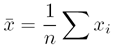
Mean:

Technically, the mean (denoted μ), can be viewed as the most common value (the outcome) you would expect from a measurement (the event) performed repeatedly. It has the same units as each individual measurement value.

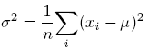
Variance:

The variance (denoted σ²) represents the spread (the dispersion) of the repeated measurements either side of the mean. As the notation implies, the units of the variance are the square of the units of the mean value. The greater the variance, the greater the probability that any given measurement will have a value noticeably different from the mean.

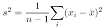
Standard deviation:

The standard deviation (denoted σ) also provides a measure of the spread of repeated measurements either side of the mean. An advantage of the standard deviation over the variance is that its units are the same as those of the measurement. The standard deviation also allows you to determine how many significant figures are appropriate when reporting a mean value.

It is also important to differentiate between the population mean, μ, and the sample mean, .

Population versus Sample Mean & Standard Deviation:

If we make only a limited number of measurements (called replicates), some will be closer to the ‘true’ value than others. This is because there can be variations in the amount of chemical being measured (e.g. as a result of evaporation or reaction) and in the actual measurement itself (e.g. due to random electrical noise in an instrument, or fluctuations in ambient temperature, pressure, or humidity.)

This variability contributes to dispersion in the measured values; the greater the variability (and therefore the greater the dispersion), the greater the likelihood that all the measured values may differ significantly from the ‘true’ value.

To adequately take this variability into account and determine the actual dispersion (as either the standard deviation or variance), we would have to obtain all possible measurement values – in other words, make an infinite number of replicate measurements (n → ∞). This would allow us to determine the population mean and standard deviation, μ and σ

This is hardly practical, for a number of reasons! The general approach is therefore to perform a limited number of replicate measurements (on the same sample, using the same instrument and method, under the same conditions). This allows us to calculate the sample mean and standard deviation, and s.

The sample mean, standard deviation, and variance (s²) provide estimates of the population values; for large numbers of replicates (large n), these approach the population values.

Exercise 1: Calculating the mean

The sample mean is the average value for a finite set of replicate measurements on a sample. It provides an estimate of the population mean for the sample using the specific measurement method. The sample mean, denoted , is calculated using the formula:

Suppose we use atomic absorbance spectroscopy to measure the total sodium content a can of soup; we perform the measurement on five separate portions of the soup, obtaining the results 108.6, 104.2, 96.1, 99.6, and 102.2 mg. What is the mean value for the sodium content of the can of soup?

You have already used the relevant Excel™ functions for this calculation in a previous exercise. Set up a new worksheet and calculate the mean value, using (i) the COUNT and SUM functions, and (ii) the AVERAGE function; you should get the same values.

Exercise 2: Calculating the variance

We also need to determine the spread of results about the mean value, in order to provide more specific information on how many significant figures we can attribute to our sample mean. We can do this by calculating the sample variance, which is the average of the squared difference between each measurement and the sample mean (i.e. the average of the squared residuals):

Note that we use a factor of (n − 1) in the denominator, rather than n. A simple justification for this is that it is impossible to estimate the measurement dispersion with a single reading – we would have to assume that the spread of results is infinitely wide. When n is sufficiently large so that n ≈ (n − 1), the sample mean and variance approximate the population values and we can use the equation:

As noted in the introduction, it is more convenient to use the standard deviation, which is simply the square root of the variance, . The advantage of using standard deviation over variance for describing your results is that s has the same units as the mean value.

Use the worksheet from exercise 1 to also calculate the variance and standard deviation of the sodium values by setting up a formula. You will need to create a column to calculate individual values of before calculating s² and s. Compare your standard deviation and variance with those calculated using the built-in STDEV and VAR functions. To calculate a square root in Excel, either use the “^0.5” notation, or the SQRT function.

Reporting Results:

The final value for the sodium content of the soup would be written as:

C = 102.₁ ± 4.₇ mg (mean ± s, n = 5)

Note that a single value, or a mean value without any indication of the sample variance or standard deviation, is scientifically meaningless. Note also that the first non-zero digit of the standard deviation identifies the least significant digit of the mean. That is, the standard deviation determines the correct number of significant figures. In our example above, for example, the leading non-zero digit in s is in the first place to the left of the decimal point, so the mean concentration is known to 3 significant figures. Finally, due to the way it is calculated a standard deviation technically only has 1 significant figure. It is customary, however. to show the first non-significant digits in both the mean and standard deviation in order to avoid rounding errors in any subsequent calculations.

Continue to Errors & Residuals...